


Consultant
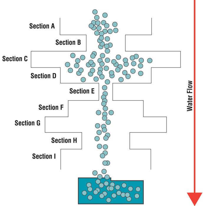
Figure 1
This shows the basic concept behind the theory of constraints. To increase flow in this
gravity-fed piping system, you would need to increase the diameter of Section E, the
constraint.
Imagine a manufacturing process in which similar machines grouped together perform similar operations. Work moves in sequence between these operations and sometimes flows back the way it came—deburring to welding and back to deburring, for instance.
This is the classic job shop, where high-mix, low-volume production simultaneously handles assorted jobs using shared resources. The jobs usually have different routings and due dates with dissimilar priorities, production quantities, and material and resource requirements.
Problems begin to surface for a variety of reasons. Things like material supplies being delayed, customers changing their quantities or due dates, machine breakdowns, and quality issues can aggravate and slow product flow. When this happens, we usually see a buildup of work-in-process (WIP), which extends lead times and delays deliveries. When this happens, the finger-pointing begins. We blame a host of factors, like customers changing their minds and priorities, suppliers not delivering materials on time, or faulty maintenance practices creating equipment downtime. But are these the true root causes, or could it be something much more basic?
To cope with these late deliveries and the resulting unhappy customers, job shops use a variety of countermeasures in their production control and operations management systems. Both Six Sigma and lean manufacturing are excellent in their own right, but if the same problems continue to plague organizations, is something missing?
If this is the case, you may want to consider another improvement method called the theory of constraints, or TOC.
Implemented correctly, the method can help simplify scheduling and improve on-time-delivery performance.
The basics can be boiled down to a simple analogy. Figure 1 shows a simple diagram of a gravity-fed piping system for water, with each section having a different diameter. Say you need to increase water flow; what would you do and why would you do it? Remember, it’s gravity-fed, so increasing water pressure is not an option.
The correct answer is that you would have to increase the diameter of Section E because it is limiting the flow of water through the entire system. But how would you decide how large to make Section E’s diameter? The new diameter of Section E would be completely dependent upon how much more water is needed. In other words, what is the new demand requirement?
Increasing the diameter of any other section of pipe would not deliver any more water because Section E is constraining the output and therefore controls the output of all the water in this system. Figure 2 shows the same piping system with Section E’s diameter enlarged, and, as you can see, more water is clearly flowing. Section B is now the constraint—or, in TOC parlance, the system constraint.
Figure 3 represents a simple linear manufacturing process. If you needed to increase output, the only way to do so would be to shorten Step 3’s cycle time to a level that would satisfy demand. Shortening the cycle time of any other step would not increase overall output. Like Section E in the piping system, Step 3 is the system constraint that controls the rate at which products can be made.
So how do these concepts simplify scheduling and aid on-time delivery? To understand this, we need to discuss how exactly TOC defines throughput. When it comes to scheduling, this definition changes everything.
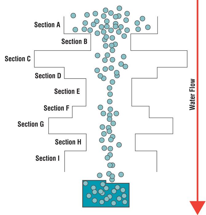
Figure 2
With Section E enlarged, more water flows through the system and Section B becomes
the constraint.
One of the pitfalls of traditional cost accounting is the mandate to keep all machines and workers busy all of the time as measured by utilization and efficiency. Both of these metrics are good, but only if measured within the confines of the constraint. Maximizing utilization and efficiency for every process on the floor only serves to drive WIP to unacceptable levels, hindering part flow and on-time delivery.
TOC challenges cost accounting’s mandate to keep people and machines running all the time. It doesn’t suggest to replace cost accounting and generally accepted accounting practices (GAAP), which is required by law, but TOC does promote adding another method that places the emphasis squarely on throughput. It’s called throughput accounting.
According to TOC, throughput is not simply the number of parts passing through a process and on to shipping. Instead, TOC defines throughput as the sales dollars received minus the total variable costs (TVCs), such as raw material costs; sales commissions; shipping charges; and outside services like heat treating, powder coating, or plating. In other words, TVC is anything that varies with the sale of a single unit of a product. Throughput accounting helps managers make real-time financial decisions that affect the company’s bottom line.
TOC uses two other metrics to judge decisions that affect the company’s profitability: investment and operating expenses. Investment represents all the money spent on things the company intends to sell; this typically includes both WIP and finished-goods inventory. Operating expenses include all the money the company spends, including all labor expenses, to turn investment into throughput—and throughput is king. Throughput accounting uses these calculations to determine net profit and return on investment (ROI):
Net profit = Throughput – Operating expenses
ROI = (Throughput – Operating expenses) ÷ Investment
So why is focusing on throughput so important? Throughput has no upper limit! As long as you have demand for your products and you successfully shorten time on the constraint (or control point), throughput will continue to grow, and so will your net profit and ROI.
TOC was developed by the late Dr. Eli Goldratt in the early 1980s, when companies didn’t have sophisticated information systems, such as enterprise resource planning (ERP) software. For this reason, Goldratt developed a simple, TOC-based scheduling method known as drum-buffer-rope (DBR). The fundamental assumption behind DBR is that every process or system has a constraint within it that controls the throughput rate of the process or system, and that production schedules should be developed based on the output of the system constraint.
It also assumes that most of the time the other resources possess sufficient capacity to support a constraint-based production schedule. Just like the piping system, the constraint may change over time, but one will always exist. In a job shop, the constraint changes from job to job, so to counter this changing of the constraint, we can designate one of the process steps as a control point—a designated constraint, if you will.
Buffer management addresses the inherent variation that interrupts work flow. Together, DBR and buffer management enable the scheduling of jobs on the constraint, based on the due dates. Because the constraint controls the throughput rate of the entire operation, we must always keep the constraint busy while controlling and limiting WIP. This is accomplished by releasing new jobs into the system only when something exits the constraint. In effect, we must pull the jobs in, rather than push them in, by scheduling the constraint. Therefore, job loading times are based entirely on the constraint’s schedule.
Of course, in any process things happen that interrupt product flow. Maybe the right material doesn’t always arrive at the right place at the right time, or unexpected downtime occurs in front of the constraint. For this reason, we need to absorb these bumps with some kind of buffer. DBR inserts strategically placed buffers in front of the constraint (control point) and in front of shipping to protect delivery due dates.
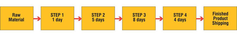
Figure 3
In this linear manufacturing process, Step 3 takes the longest and so represents the constraint.
Buffers are necessary to account for process variation, but we don’t want to clog the system with excess WIP either. For this reason, we base these buffers on the time it takes for a new part to arrive at the constraint operation. The buffer absorbs and dampens the ever-present negative effects of system variability.
Say a fab shop identifies welding as its control point. One job flows through laser cutting, deburring, and then bending before it gets to the welding control point. It takes two hours for the first kits to flow through those upstream processes and arrive at the first welding cell. After two more hours of production, 30 more kits arrive in welding. So in this instance, the number of kits in the buffer should be based on what can be produced in two hours—30 kits of parts. Anything less, and you risk starving your constraint operation. Anything more, and you’re flooding the floor with excess, costly WIP.
When there is a bump in the system—and there will be many bumps—buffers make it easier to overcome and absorb those bumps before they cause a problem at the constraint or in shipping, reducing the throughput rate. These strategic buffers make DBR a robust, reliable way to account for process and product variability.
The buffers also help build awareness of problems in the process, those “things” that seem to eat holes in these buffers time and again. Because you monitor these buffers, your company will know where to focus improvement efforts.
Figure 4 shows the same process layout as in Figure 3, only now we’ve implemented DBR. We’ve identified the constraint as Step 3, and since we never want to starve that constraint operation, we’ve added a buffer in front of it.
To avoid this excess WIP, we send a signal (the rope) to the initial process (sometimes called the gating process) to begin a new part when a part exits the constraint (the drum), which sets the pace for the entire operation. Similarly, we add a buffer and rope in front of shipping to protect against orders being shipped late. The rope’s signal in this case is sent back to the constraint.
The three buffer colors—green, yellow, and red—act like traffic signals for the shop floor. If a part exits Step 2 on time, it is within the green zone and no action is required. If a part is late exiting Step 2, it falls into either the yellow or red zone depending on how late it is. Yellow would indicate that we should check the status of the late part and develop a plan to expedite it. If it falls into the red zone, then the plan to expedite must be implemented or the part will arrive at the constraint late.
One more component must be implemented for any successful improvement initiative: the active involvement of front-line workers, the true subject-matter experts.
Rather than being a token member of the improvement team, your front-line workers need to be provided with the full DBR/buffer management training package, and you must listen to and implement their ideas. If you follow this guideline, your front-line workers will own the solutions, and they will do whatever it takes to make your DBR initiative successful.
If your company has an MRP or ERP system in place, it can still be put to good use for scheduling using DBR. There are a number of ways to do this depending upon whether the environment is a job shop or repetitive operation, and whether the MRP lead times are fixed or dynamic.
DBR has helped improve throughput and on-time delivery while controlling WIP. It has worked well in job shops, hospital emergency rooms, even MRO companies. It works because it changes your production scheduling system from “push” to “pull.” It is this simple change that dramatically improves flow. When improvements are made to flow, great things happen for your company and your customers.
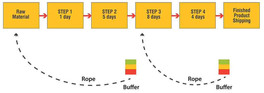
Figure 4
To avoid excess WIP, when a product exits the constraint process, drum-buffer-rope scheduling sends a signal to the initial process to release an order into the system. An inventory buffer is also placed before shipping. In this case, the rope’s signal is sent back to the constraint process.
The Fabricator is North America's leading magazine for the metal forming and fabricating industry. The magazine delivers the news, technical articles, and case histories that enable fabricators to do their jobs more efficiently. The Fabricator has served the industry since 1970.
start your free subscription
Easily access valuable industry resources now with full access to the digital edition of The Fabricator.

Easily access valuable industry resources now with full access to the digital edition of The Welder.

Easily access valuable industry resources now with full access to the digital edition of The Tube and Pipe Journal.

Easily access valuable industry resources now with full access to the digital edition of The Fabricator en Español.
In this episode of The Fabricator Podcast, Caleb Chamberlain, co-founder and CEO of OSH Cut, discusses his company’s...