


The tipping point: A new way to manage value streams in high-mix manufacturing
A new VSM method has big potential for the job shop

Eliminating waste is everyone’s job. For the past few decades, the tool of choice in waste elimination has been value stream mapping, or VSM. The universally accepted methodology for this technique is described in John Shook’s book Learning to See (that is, learning to see waste). Shook’s process is elegantly simple and easy to learn. Results are easy to interpret and can be used to document the current state as well as provide a vehicle to map the future state or desired condition.
The importance and impact of a team’s ability to rapidly generate a simple, visual conceptualization of a process flow using Shook’s spiral-bound workbook cannot be overstated. The methodology is particularly relevant when mapping a highly repetitive process, such as building cars.
Those who work at job shops, though, often vent significant frustration when attempting to map a constantly changing order file and nearly infinite number of product flows. From my experience, when people need to erase and recalculate VSM data repeatedly, they throw up their hands in surrender, assuming that VSM (and possibly lean manufacturing) is not a viable approach in their high-product-mix world.
Ten years ago I experienced a tipping point in this area. I was working in Canada at a company producing oil pipeline equipment. They had previously hired a lean consultant familiar with the Toyota model and he (in their words) “dogmatically demanded that they set up their value streams using the TOP methodology [takt time, one-piece flow, pull system].” One value stream produced well head casings, which are large pieces of pipe with one, two, or three flanges. These 200-pound pieces of hardware were turned on a large lathe. Then they were drilled, cleaned, painted, and shipped to a job site where they were bolted or welded to a piece of pipe sticking out of the ground atop a freshly drilled oil well.
The traditional Learning to See method was used to develop the current- and future-state maps. Unfortunately, the mix of sales orders changed daily, and the work content (operator and machine cycle times) varied so much that they were constantly over- or understaffed. They eventually abandoned the consultant’s recommendations. They were willing to try again after hearing me speak at a FABTECH® conference. However, when I visited, they were very prescriptive: “Don’t talk to us about takt time,” they demanded. “We have tried it already, and it does not work here.”
They were correct. The traditional takt time and VSM process would not work in their highly volatile production system. I knew that I would need to develop an alternative to the widely accepted method. From that I have refined a new, robust, scalable, flexible VSM tool for helping any company learn to see and eliminate waste.
Identify the Value Streams
Let’s say we work at a fictional high-mix, low-volume shop. Because our products differ based on material type or require different routings (some parts get grained or have hardware installed), we first have to determine if there is enough demand to constitute multiple value streams.
Let’s assume we have one laser and one punch. The fact that not all parts go through all processes is OK. We expect that, and our VSM process accounts for a variety of routings.
Also, before developing a map, we must determine the unit of measure. The entire VSM should use the same (common) unit of measure, whether that is pounds, lineal feet, tons, or pieces. The same applies to time. If your processes are long, you may decide to represent time in hours; if the process times are short, then minutes or seconds. Try to keep the same unit of measure throughout.
In the example that follows, we’ll use the number of pieces as the unit of measure and seconds when measuring time.
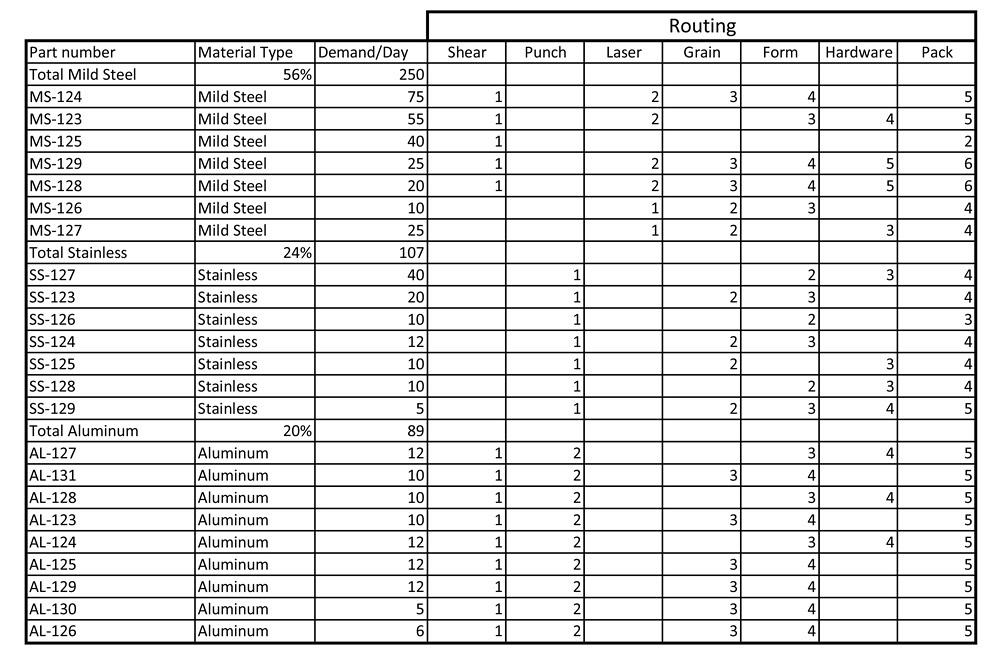
Figure 1
This product-quantity-routing analysis sorts jobs by material type. It appears a significant number of like-material jobs have the same or similar routings.
For this example, we will use fewer than 25 part numbers. Most job shops have many more active part numbers than this, so keep in mind that performing this sorting process is likely to take a bit more effort. Also, for the sake of simplicity, we assume that these jobs involve cut and formed sheet metal parts that require some hardware insertion but no welding or assembly. The routing steps are cutting, graining, forming, hardware insertion, and shipping.
The first tool we use to determine the value stream is a product-quantity-routing, or PQR, analysis. Another way of saying this is: P = What we make, Q = How much we make, and R = What processes are used to make it. The PQR analysis may determine that the value streams are customer-focused, material type-focused, product size-focused, quality requirement-focused, or machine capability-focused.
For this product mix, it appears that grouping jobs by material type may work best (see Figure 1). While there is some minor variation in routings within a material type, it appears that mild steel products tend to flow primarily the same path, while stainless and aluminum flow a path that’s closer to each other’s than to mild steel’s path.
Mild steel represents the greatest percentage of work (56 percent), while the combined demand of stainless steel (24 percent) and aluminum (20 percent) are about equal to mild steel. Since stainless and aluminum are both processed on the punch, we will divide the work into two value streams: mild steel (laser-cut parts) and stainless/aluminum (punched parts).
Note that the decision of whether to set up three smaller value streams rather than two larger ones is an important one. It must be based on how many machines you have and how likely it is that downstream operations have the capacity to maintain flow.
Here we’ll assume downstream operations can handle two value streams, and from here on we’ll focus on just one: the mild steel value stream. We’ll also assume that this value stream consists of cross-trained workers capable of carrying pieces through multiple steps: laser, graining, forming, and hardware insertion.
Demand, Takt Time, and Flow
First, we need to determine demand. Most OEMs can reasonably predict demand; therefore, changes to takt time may be infrequent. Job shops, though, must manage quantity variations throughout the week, month, and year, resulting in more frequent adjustments to takt time, or the manufacturing rhythm.
For this example, we will assume a constant daily demand of 250 components: 125 computer chassis components and 125 go-cart components. The computer chassis components require hardware insertion, while the go-cart components do not. This will mean a difference in the product flow and staffing associated with that operation, which will likely be a shared resource with the stainless/aluminum value stream.
Next we need to know the available time. We have 480 available minutes (8 hours) over one shift, not counting 10-minute breaks, which I’ll address later. To determine takt time, we divide available time (AT) by demand (D): AT/D = Takt time. We divide 480 by 250 to get a 1.92-minute takt time. Our common unit of time is seconds, so we multiply this by 60 to get a takt time of 115.2 seconds.
Knowing this, we need to develop a system to produce a unit (component) every 115.2 seconds—or less than 2 minutes. This value will be used throughout the VSM to determine the appropriate number of people, machines, space, plant layout, and inventory levels to meet that goal.
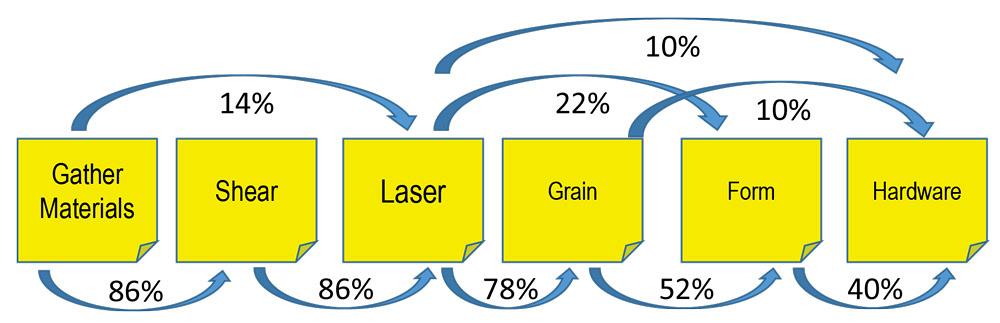
Figure 2
This flow chart shows what percentage of pieces in the mild steel value stream share a specific routing. For example, 14 percent of parts move from raw stock (gather materials) to the laser, while 86 percent go from raw stock to the shear and then to the laser.
Labor content divided by takt time indicates how many people are required to maintain the required output. To be clear, the labor content of a process may be well over 115.2 seconds per unit. Labor content and takt time are two different things. If the labor content is less than 115.2 per unit, then we would need one person to spend at least part of his or her day to accomplish the task. If the labor content is more than 115.2 seconds per unit, then we would need more than one person.
Using Post-It notes and a large wall or whiteboard, we show the process in a flow chart, including all the major variations and percentages of flow—that is, what percentage of pieces in the value stream share that specific routing path. As the flow chart in Figure 2 shows, 86 percent of pieces go from raw stock to the shear and then on to the laser, while 14 percent go from raw stock directly to the laser.
If you can’t identify a unique flow for all of your products, don’t agonize over it. Job shops can’t hope to map 100 percent of everything they do. Leave out the minor product categories. Otherwise you will “what if” yourself into static inertia.
Process Boxes
For each process we then fill out a form—what we’ll call a process box—that includes the operator cycle times, machine cycle times, setup times, the distance traveled per unit, and current work-in-process (WIP) inventory (see Figure 3). Later we will develop a future-state map that reflects the true WIP levels required to maintain output at the takt time.
In practice, you need to account for the true workstation load. For instance, working from the flow chart in Figure 2, we see that the shear processes only 86 percent of our pieces. Workstations also may process work from other value streams, which needs to be accounted for as well.
But just to introduce the process box concept, we’ll keep the math simple and assume that except for hardware, all 250 parts for the day are routed through every process in the mild steel value stream.
For most processes, we determine the operator cycle time and setup time with some simple time studies, observing and recording how long it takes operators to perform certain tasks. When an operator retrieves a raw sheet to put in the laser, though, we run into problems. He’s not processing just one part or product, but instead an entire sheet that will be cut into a nest of blanks.
So to obtain the operator cycle time for the “gather materials” step, we go by the average lot size in the value stream. Based on information from Figure 1 (averaging the numbers in column 3), the average lot size within the mild steel value stream is 35 units, so setup times, gather materials, and other activities performed once per job will be divided by 35. We’ve determined we need 5 minutes to gather enough sheet metal for 35 units. So we divide 5 by 35 and get 0.143 minute, or 8.57 seconds, as shown as the weighted-average operator cycle time (OCT).
The critical numbers in the process boxes are the weighted averages of OCT, machine cycle time (MCT), and setup time (SUT). That’s because unlike product-specific value streams, our mild steel value stream handles different products, and the mix might change each day. For gathering materials, the cycle time for both computer chassis and go-carts is the same. But for most processes, the cycle time will differ depending on the product, which is why we need to work from weighted averages.
To determine the operators required for a particular process, we add the total labor input for the process—that is, the weighted averages of OCT and SUT—and divide by our takt time of 115.2 seconds. Laser cutting, for instance, has a weighted average OCT of 37.5 seconds and SUT of 15 seconds (again, this is per piece). So here, we get (37.5 + 15)/115.2 = 0.4557, which we round up to 0.5.
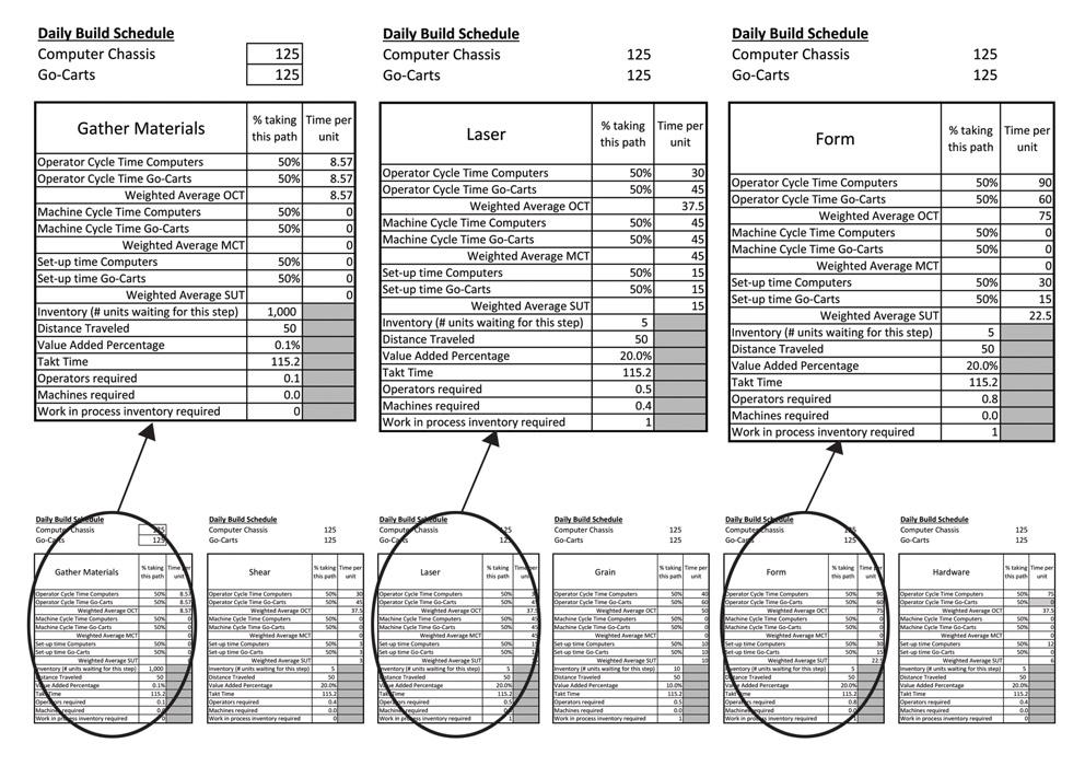
Figure 3
For every step in the flow chart, we create a process box that details the average operator cycle time (OCT), machine cycle time (MCT), and setup time (SUT). To illustrate the details, three process boxes—gather materials, laser cutting, and forming—are magnified. To figure the operators required for a particular process, we add the weighted averages of OCT and SUT, then divide by the takt time (115.2 seconds). Similarly, for required machines, we divide the weighted average MCT by the takt time. Forming has zero MCT because our shop’s manual bending process does not run independently, without an operator. The MCT is accounted for in the OCT.
You’ll notice in Figure 3 that for forming our machine cycle time is listed as zero. This is because the manual machine doesn’t run independently of the operator cycle time, so we don’t need MCT in our analysis. As this shows, we need 0.8 (round up to 1) operator, so we obviously also need one press brake. The same reasoning applies to hardware insertion.
When we add up the operator values in all the process boxes in the value stream (see Figure 4), we find that on this particular day, with this particular product mix, we have a required staffing level of 2.6, which we’ll round up to 3.
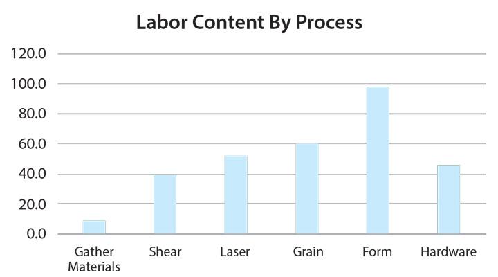
vStaffing with three people probably isn’t sufficient, though. Again, we run a job shop, and as such we need to deal with imbalances between work content of each process. Figure 5 shows the labor content (weighted average OCT + SUT) of each process. For every process we have a healthy buffer except one: forming. The press brake operation takes almost 100 seconds to form the components for one unit (75 OCT + 22.5 SUT = 97.5). This again is an average of a variety of actual cycle times, so we’re really in danger of exceeding our 115.2-second takt time.Staffing the value stream with just three people doesn’t leave much room for error. When we add up all the average labor times—that is, the average OCTs and SUTs—from every process box in the value steam, we find that this particular mix of products has an average of 302.6 seconds of labor, or just over 5 minutes. Divide this by three people, and we get a little more than 100 seconds of work each to perform a 115.2-second takt time.
This may be doable in a highly predictable assembly line, but it’s a bit more challenging in a job shop, where the work content varies so much from product to product. Moreover, people don’t work every second of every day, so we need to account for breaks and other activities. For this reason, it’s a good rule of thumb to load each person to no more than 85 percent of his or her capacity during a shift. We also want to drop that percentage a bit for each additional work assignment. For this reason and others, we might be wise to staff this value stream with up to four people.
Assigning Standard Work
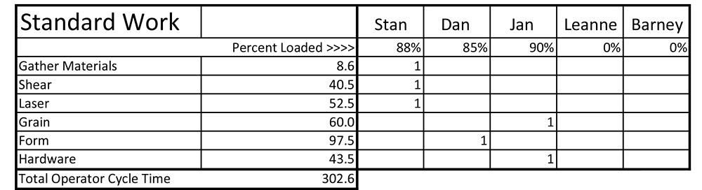
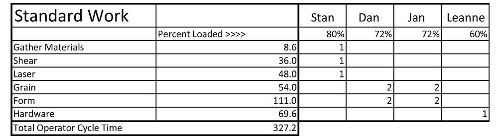
This problem becomes abundantly clear when we assign standard work—that is, work each person does each takt time or cycle. Figure 6 shows the standard work for a team of three, plus the total labor content cycle time (average OCT and SUT from Figure 6) for each process step. If Stan’s job is to gather materials (8.6 seconds), run the shear (40.5 seconds) and the laser (52.5 seconds), that gives him a total cycle time of 101.5. In other words, he’s loaded to about 88 percent of his total work capacity, which is high.
Overcoming the Job Shop VSM Conundrum
All this sounds great, but again, no job shop processes the same product mix day after day, month after month. Customer demand changes, as does the product.
Here is where this VSM approach really shines. If we have the formulas set in Excel or similar software, we can change certain variables and then redistribute the standard work. Say our volume stays the same (250 units) but now you have 200 computer chassis (80 percent of total) and 50 go-carts (20 percent). Because we’re still producing 250 units a day, our takt time doesn’t change. But the change in product mix does change our cycle time averages, increasing the total work content from 302.6 seconds to 327.19 seconds. Being able to quickly adjust the work content to balance the line may mean having a very flexible workspace (see Figure 7).
Entering 1 beneath a person’s name assigns all of the work of a particular process to one person; entering a 2 splits that time in half; entering 3 divides the time into thirds, and so forth. If you enter a 2 under Dan’s name in this case, don’t forget to enter a 2 under someone else’s work assignment—in this case, Jan.
Achieving Steady Flow
Dividing the activities into logical buckets of work that each person can accomplish within each takt time helps define and maintain a steady flow of products. Where there is a highly volatile change in mix each day, this tool can be invaluable in determining how many people are needed and where they are best deployed.
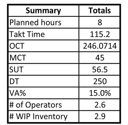
Figure 4
This shows the totals from all the process boxes in Figure 3, including the average operator cycle time (OCT), machine cycle time (MCT), setup time (SUT), and distance traveled (DT). Add total MCT and SUT, and you get a total labor input of 306.2 seconds.
We also can determine the shop layout depending on who is assigned which tasks. Most shop layouts are determined by where the open spot was on the day each machine arrived. Often, little or no thought is given to how flow will be affected. In this example, if Stan is assigned the activities of gathering material, shearing, and laser cutting, then it makes sense that these operations be positioned close to each other.
This value stream method has been a tipping point for many make-to-order shops where a standard product is not a reality. If you are one such shop, and the traditional VSM system doesn’t work for you, give this method a try.
Mapping Makes a Difference at McKenna
McKenna Metal, a precision sheet metal shop in Portland, Ore., is housed in a 15,000-square-foot brick building just a few miles away from the confluence of two major rivers, the mighty Columbia flowing south from the Canadian border and the winding Willamette.
McKenna Metal is also at the confluence of two major external influences related to its business. First, customers want their products on time, at a low cost, and with the highest quality. Second, changes in the competitive landscape have begun eroding margins and profitability.
When Scott and Rosalind (Roz) McKenna expanded their home-based business into their current location in 2009, they had relatively few competitors for their highly customized work. In the face of an economic downturn, hungry competitors losing juicy high-volume work turned their attention to customers who needed prototypes, one-offs, and low-volume orders.
For McKenna Metal, survival meant turning to lean manufacturing as a vehicle to extract waste from its processes. Through an engagement with the Oregon Manufacturing Extension Partnership (OMEP), McKenna Metal applied 5S (workplace organization), TPM (total productive maintenance), setup time reduction, and initial value stream realignment.
It also implemented value stream mapping (VSM). What successes has McKenna Metal had? It has reduced overtime and helped it avoid expanding into a second building. Ultimately, this eliminated the need for a second shift. The company is able to understand its value streams, make adjustments accordingly, and excel at meeting customer demands.
This can be your company’s story too.
About the Author
About the Publication

subscribe now
The Fabricator is North America's leading magazine for the metal forming and fabricating industry. The magazine delivers the news, technical articles, and case histories that enable fabricators to do their jobs more efficiently. The Fabricator has served the industry since 1970.
start your free subscription- Stay connected from anywhere

Easily access valuable industry resources now with full access to the digital edition of The Fabricator.

Easily access valuable industry resources now with full access to the digital edition of The Welder.

Easily access valuable industry resources now with full access to the digital edition of The Tube and Pipe Journal.

Easily access valuable industry resources now with full access to the digital edition of The Fabricator en Español.
- Podcasting

In this episode of The Fabricator Podcast, Caleb Chamberlain, co-founder and CEO of OSH Cut, discusses his company’s...
- Trending Articles
1
AI, machine learning, and the future of metal fabrication

2
Employee ownership: The best way to ensure engagement

3
Dynamic Metal blossoms with each passing year

4
Steel industry reacts to Nucor’s new weekly published HRC price

5
Metal fabrication management: A guide for new supervisors