Tube Hydroforming Design Flexibility—Part VIII: Dimensional Stability

Tubular automotive structures commonly have been made by joining several stamped parts with GMAW or spot welding, which achieves a reasonable balance of part design flexibility and hole placement. However, assembly and weld distortions create more variability than is desired. Tube hydroforming eliminates both operations and significantly lowers variability. With hydroforming, tolerances of 1/4 or less than those found in stamped and welded assemblies and higher capability levels can be achieved.

It is important to understand that a complete description of a part feature's dimensional stability must include the tolerance and capability level being maintained. When either is discussed or specified without the other, the information essentially is meaningless. The part and its feature being considered, its datums, production rate, and the sampling period also can have an effect on what the numbers represent. Attention to these details is important, since short- versus long-term data and measured range rather than statistically calculated range at a specified capability level can give attractive low numbers, but represent only part of total variation.

Figure 1

In the tube hydroforming industry, some claims treat the range of observed readings from a part population as being equivalent to statistically calculated process capability. This is false, because the former is what you see and is usually much smaller than the latter; inspection normally does not detect samples at the measurement distribution's outer limits.

To clarify misconceptions such as this, it is helpful to review related terminology, even though doing so may be redundant to some.

The normal distribution shown in Figure 1is typical of those found in statistics textbooks. It shows the actual measurements grouped into histogram bars and the normal distribution curve approximated from them. The vertical lines define capability zones, the proportion of the population in each zone, and the predicted part defect rate.

A key point to understand is the difference between the range of measurements and the statistically calculated variance at a given capability level (for example, C p = 1.33). This variance expresses the feature size range or tolerance needed to encompass the proportion of measurements that are required to achieve the desired capability level (for example, 99.994 percent at C p = 1.33). The data range from a parts group—no matter how large the sample size—will be significantly smaller (normally less than half) than the necessary tolerance. Examples showing this are detailed below.

C p is discussed rather than C pk because the former is a pure measure of variation, and C pk expresses variation combined with the data's mean value relative to nominal or CAD model position.

Figure 2	Figure 3

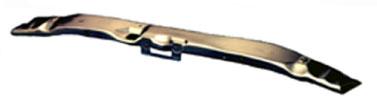
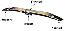
Data from the surface location in an engine cradle's unbent section (see Figures 2, 3,and 4) illustrates this point. The tolerance is ±1.0 mm, range is 0.35 mm, C p = 4.28, and the span between datums is 840 mm.

C p = 4.28 is approximately equal to ±12.5 s, which is far beyond what could ever be needed. With the capability level of C p = 1.33, or ±4 s, the tolerance that can be achieved theoretically falls proportionately to ±0.31 mm. This calculation offers a simplified way to assess the sometimes confusing interaction between the tolerance and capability. At a normal capability level, the tolerance that can be achieved is lower for stable features such as this. Maintaining this feature tolerance dimension requires a little extra breathing room—in this case, perhaps ±0.4 or ±0.5 mm.

If a tolerance is provided without the capability level, the proportion of the total population encompassed is unknown. Similarly, if the capability level is given but not the tolerance, it is unknown how large the tolerance needs to be for the capability level.

In the table in Figure 4, the capability level of C p = 1.33 was chosen for long-term data, because it is the most demanding common requirement for automotive part production. A higher capability level increases the needed tolerance, and lower capability reduces the tolerance that can be achieved. For most of the features presented, the data provided is long-term, because it obviously is preferable.

Following are three additional examples of the tolerances for different part features formed by pressure sequence hydroforming (PSH). The part type, shape and measurement data, and statistical values are described. These values include capability at the tolerance specified and, most important, the achievable tolerance at a "normal" long-term capability level of 4 s.

	Sample Period 6 Months Sample Size 30 pcs. Tolerance ±1.0 mm Range 0.09 mm Std. Dev. 0.024 C p 13.60 C pk 12.35 At C p = 1.33 Tol. = ±0.10 mm
Figure 5	Figure 6

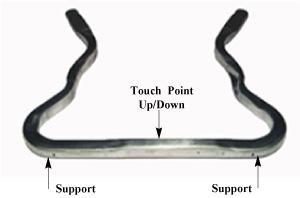
A hydroformed engine cradle cross-section width is shown in Figure 5. Figure 6shows hydroforming's precision. It uses 63.5-mm (2.5-in.) dia., 2.0-mm minimum wall thickness tubing, and the material is 45,000-PSI minimum-yield high-strength low-alloy. Keep in mind that the table presents only part of the position information usually required. A cross-section's size normally is not as important as where those surfaces are located in space relative to a CAD or nominal position. It is applicable mainly when the surface location opposite a datum is critical or a bracket fits around the tube and is located relative to the cross-section.This feature is from the part shown in the preceding example.

It also illustrates how an impressive tolerance can be indicated, in this case even with a capability level, but unless you understand the low variability nature of this feature, you could assume that such tolerances are normal on most features on hydroformed parts, which is not true.

	Sample Period 2.5 Months Sample Size 185 pcs. Tolerance ±1.5 mm Range 0.40 mm Std. Dev. 0.04 C p 11.45 C pk 9.98 At C p = 1.33 Tol. = 0.16 mm
Figure 7	Figure 8

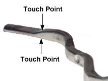
For a radiator enclosure surface location (Figure 7), the high C p shown in Figure 8results from the higher-than-normal ±1.5-mm tolerance and excellent repeatability. Production during this period was 80,000 pieces.

This result is remarkably consistent because the span is 1,260 mm. The tolerance at C p = 1.33 is ±0.16 mm. The tube is 76-mm (3-in.) dia., 1.3-mm minimum wall thickness, and the material is SAE 1008/1010 galvanneal.

	Sample Period 3 Months Sample Size 1000 pcs. Tolerance ±1.5 mm Range 1.10 mm Std. Dev. 0.17 C p 2.94 C pk 2.47 At C p = 1.33 Tol. = ± 0.68 mm
Figure 9	Figure 10

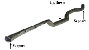
The instrument panel beam surface location before welding (Figure 9) is 50.8-mm dia., 2-mm minimum wall thickness, SAE 1008/1010 mild steel tube. Cycle time is less than 17 seconds, and volume of up to 780,000 parts per year is achieved with two shifts and a partial third. This third iteration of a part that has been in production for nine years ran in one press in a single-cavity die with no backup tooling. Manufacturing scrap rates from bending, hydroforming with hole punching in the die, and shearing totaled 0.5 percent. The tolerance and other statistics for this part run are shown in Figure 10.

The other commonly used hydroforming process, high-pressure hydroforming (HPH), is able to make similar parts, but comparable production dimensional stability information has not been presented publicly. It would be interesting to see how HPH compares to PSH in producing dimensional stability, but this cannot happen until comparable HPH data is made available. If any reader knows of such information, I would be interested in discussing it.