Why a timeline analysis of order history matters

Part 5 in a series: The traditional PQ Analysis may point job shops in the wrong direction

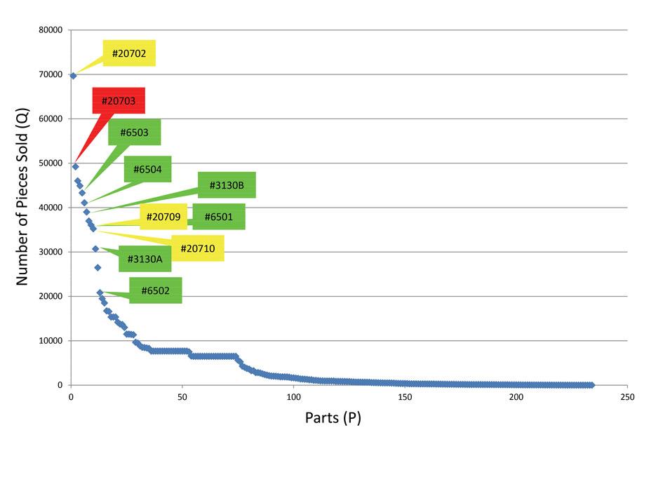
Figure 1
This PQ Analysis curve shows a typical job shop product mix, with a few parts produced in high volume (runners) and a long tail of parts produced in low volume (strangers). The horizontal axis represents part numbers, and the vertical axis represents the quantity of each part. The labels show which part numbers the shop classified as runners using only the PQ Analysis.

The traditional PQ Analysis incorporates a manufacturer’s list of different products (P) and the quantities (Q) produced of each. It helps determine which products are runners (high volume), repeaters (medium volume), and strangers (low volume). Unfortunately, it ignores details about every product’s order history, including the number of orders placed, the quantity/size for each order, and the time interval between consecutive orders. So, using the PQ Analysis alone may classify two products having identical annual shipped quantities as runners--that is, of high volume.

But what if during the past year customers placed relatively small-quantity orders for one product twice a month for every month, and for the other product placed only a single large order? If PQ Analysis were used, it would have considered only the cumulative shipment quantity for the entire year for both products. Because they have identical volumes, they would be seen as equally important. But in reality, because their demand variability (T) is so different, the shop should handle each job differently.

For the product ordered many times, with each small-quantity order requiring a short run, the shop may need to run each order on a different machine, depending on equipment availability. Or the job could be run on a single flexible, CNC machine with quick-change tooling and fixtures. For the product with a single large shipment quantity, one machine could process the entire production run. To make this order more profitable, managers could organize a kaizen to identify potential problems. They could, for instance, offer the customer a level-loaded delivery schedule, possibly by splitting the order quantity and spreading deliveries over consecutive months; this means the spike in demand imposed by this one-time order could be smoothed over a planning horizon.

Time Matters

The PQT Analysis factors in the demand variability with time (T); that is, it considers a product’s order history. This changes how a shop determines whether products are runners, repeaters, or strangers. Runners would be products having both high volume and high demand repeatability; that is, they are ordered relatively frequently at predictable intervals. Repeaters would have medium volume and medium demand variability; and strangers would have both low volume and low demand repeatability--they are ordered infrequently at unpredictable intervals.

Consider Figure 1 showing the typical “long tail” of a job shop’s product mix. The callouts show which parts this shop identified as runners. But this classical Pareto analysis does not show the whole story because, again, the analysis considers only a product’s aggregate volume over several consecutive years, not how frequently the orders for that product came in the door throughout that period.

Figure 2 brings demand repeatability (T) into the picture, showing the number of pieces ordered over the different years as well as the number of orders placed during a given year. Those who are Excel-savvy and would like to put their Six Sigma Black Belt training to the test could also record the number of pieces associated with each order, since that would give them the complete timeline needed to analyze the order history for every part (or part family) they make.

Figure 2 illustrates a timeline analysis. It really is a “quick and dirty” PQT Analysis, considering we are analyzing only the number of orders placed over several years. As stated, two products with identical annual shipment quantities may both be ordered six times in one year but ought to be treated differently if, say, one product has six orders within just two months, while the other product is ordered six times at unequal intervals spread throughout the year.

This is why using shorter time increments, such as months or weeks, can yield much more information than just a cumulative quantity for each year. This is also where in-depth statistical analyses can help, such as the time-series analytics available in Excel® or even a statistical analysis package like Minitab®. (Some in-depth analyses use coefficient of variation instead of the number of orders. For more on this, see the book Factory Physics, www.factoryphysics.com, or Peter L. King’s Lean for the Process Industries: Dealing with Complexity.)

Still, even though this quick analysis just scratches the surface, it can reveal much about reality on the shop floor. Recall the part numbers labeled as runners in Figure 1. Now look at Figure 2, which shows a more complex story. Some are ordered frequently one year, then only a few times the next year.

After eyeballing an Excel plot of a Pareto analysis of just the number of orders placed for each product, the shop decided that a stranger is a part ordered fewer than 10 times during 2004-2007; a repeater is ordered 11 to 50 times during the same four years; a runner, more than 51 times in the same timeframe.

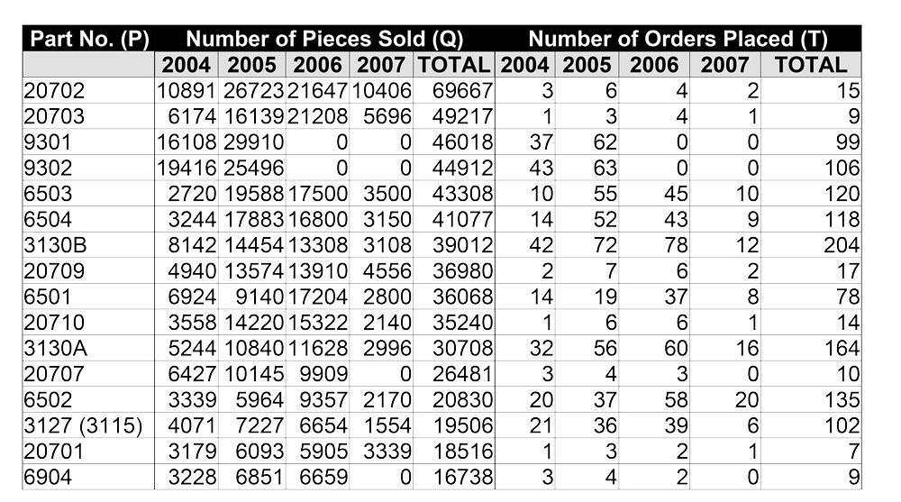
Figure 2
This partial list of products shows the quantities of products as well as how many times they are ordered during a particular year. A complete list could include hundreds or even thousands of additional products, depending on the size of the job shop or the sample size (partial list extracted from the complete active part list) selected.

The result in Figure 3 shows how the PQT Analysis completely changes how a shop segments its part mix and decides on how to do business for its runners versus its strangers. There are only half as many runners, compared to the number of runners identified by the PQ Analysis. In fact, the shop classified four high-volume products as repeaters, simply because they were ordered infrequently compared to the rest of the runners.

Part Family Cells Based on PQT Analysis

One challenge of implementing manufacturing cells in a job shop is ensuring that demand for the products produced in those cells remains stable throughout the year, possibly for several years. If demand fluctuates, then the job shop needs to either run a particular cell during certain periods of the year, then idle that cell and move its employees (and sometimes certain mobile machines in that cell) to other areas for the rest of the year, or run the cell throughout the year but rely on cross-training to vary the cell’s staffing level to match demand. The shop also can make the cell more flexible, but there are downsides to flexible cells, regardless of whether it involves more automation or more cross-training of employees.

Demand variability nullifies several key reasons a manufacturer implements cells in the first place: to foster teamwork and operate each cell autonomously as a business unit. Ultimately, cells can place decision-making responsibility in the hands of those who actually produce the value for the company.

Also, if a cell’s demand were stable, then its leader could ensure that his or her employees are trained in several critical functions that the cell requires to be operating at the highest overall equipment effectiveness (OEE). But with employees working in multiple cells, quality and commitment to cross-training may suffer. That is because a cell gives the people who work in it an identity. They see their goal as to make any and every part in this cell’s family in the right quantity with the right quality at the right time.

Selecting, training, and retaining a flexible workforce capable of working in multiple cells during any shift as demand fluctuates is no easy task. In addition, each of these employees would require access to new order details regardless of where they work in the shop. This would require the shop’s enterprise resource planning (ERP) system to carry complete and accurate documents and specifications, and that it be accessible via computer terminals or electronic displays placed at strategic locations in the facility. Of course, what is most important--and challenging--is tracking and ensuring consistent quality of work done by these flexible employees, regardless of which cell they work in.

Finally, job changeover times could increase if a cell’s part family is a mixture of runners and strangers. This can occur because of the learning effect, which guarantees that, even for the simplest of tasks, the changeover and cycle times decrease as the operator repeats the same task. The more an operator repeats a process, the better that operator becomes. The same applies to machines, tools, as well as gauges. That’s why work consistency and quality can be so high in a cell producing a part family of runners and repeaters.

The Money Value of Time

The PQT Analysis and the learning effect both affect how a job shop costs an order and determines labor and machine-hour rates, based on different levels of part complexity and volumes, performed by employees with different skills and work preferences.

In a typical job shop, much time could elapse between two orders of the same product or product family. This often means that employees must climb the learning curve each time they transition between orders that involve products from different product families. In fact, when two dissimilar jobs run consecutively on the same equipment, both the machine and its operator go through a kind of learning curve. A potential solution may come from the engineering methods of Group Technology (GT). GT is an improvement methodology pioneered by the Russians, Germans, and British in the 1960s that, when combined with time studies, can identify which attributes of each product family affect learning speed.

Job shop managers may say that each product they make is different, but if they put their minds, video cameras, ERP data, spreadsheets, and business analytics tools to work, they probably will find repeating patterns in their order history. In fact, a thorough implementation of PQR$T Analysis will lay the foundations for discovering similar or even identical patterns of work in everything they do.

This article is part of a series. For other articles in the series, click the following:

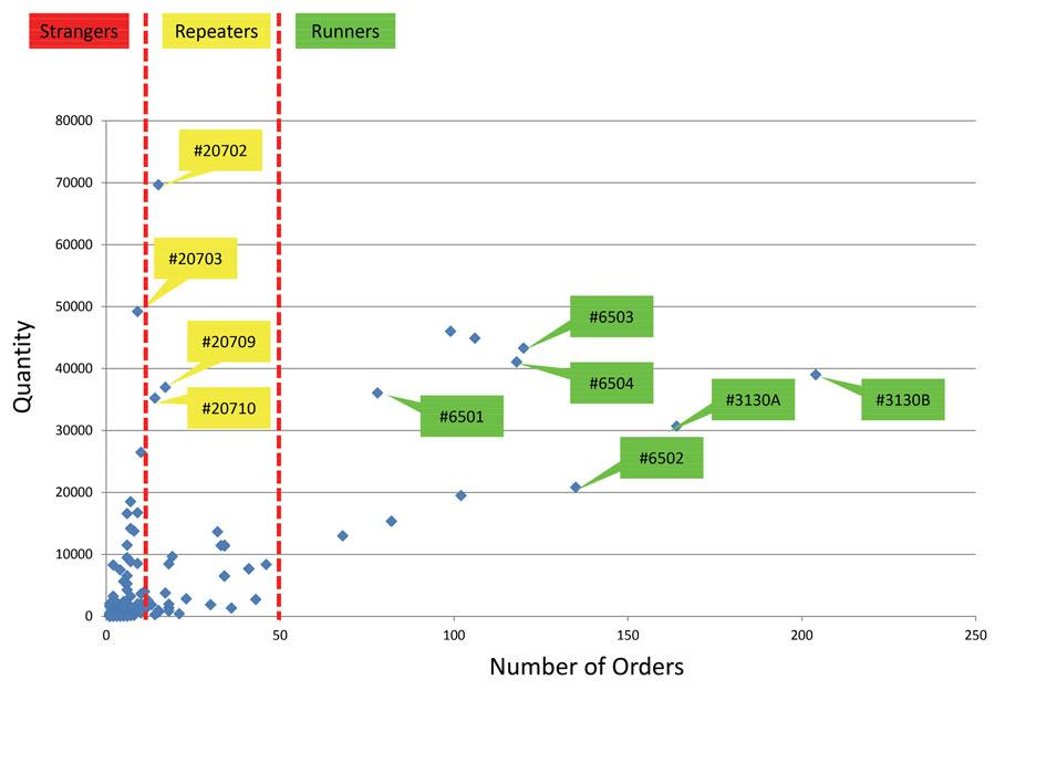
Figure 3
This complete PQT Analysis changes how the shop classifies its strangers (low volume), repeaters (medium volume), and runners (high volume).