


President
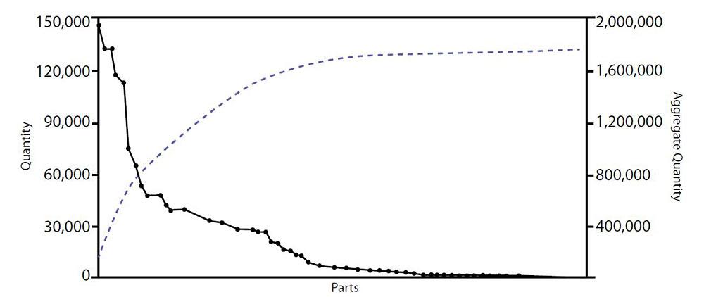
Figure 1
This PQ Analysis graph relates a job shop’s 79 part numbers to per-order quantity (left axis) and aggregate quantity (right axis).
Most job shops are the polar opposite of the Toyotas of the world. They have a diverse mix of products (P) with different routings (R) produced in various quantities (Q) with varying revenue and profits ($) and demand repeatability (T). These parameters for each different product are all taken into consideration by PQR$T Analysis, a comprehensive data analysis tool that job shops can use to perform product-mix segmentation. This ultimately helps any job shop to identify the various “businesses” it is knowingly (or maybe unknowingly) operating, from somewhat predictable repeat work to one-off prototypes.
PQR$T Analysis builds on the traditional PQ Analysis, a method for product mix segmentation that OEMs and top-tier manufacturers have embraced for years to plan their lean implementation. Typically, PQ Analysis identifies two distinct segments in a manufacturer’s product mix: those products that are in the high-mix, low-volume (HMLV) segment and those products that are in the low-mix, high-volume (LMHV) segment. The production system designed for one segment is not going to be optimal for the other segment. In fact, the use of PQ Analysis encourages a job shop to utilize value stream mapping, a lean tool that is fundamentally incapable of analyzing the HMLV segment of the job shop’s product mix. For example, the HMLV environment calls for short production runs, whereas the LMHV environment calls for long production runs, and this significantly affects a number of manufacturing factors, such as:The PQ Analysis method can be used to segment the product mix based on the annual production volume of each product. This helps determine the type of layout best suited for each segment: flow line, job shop, cellular, or some combination of these basic layouts.
The typical PQ Analysis curve for an HMLV facility will show, at the left end of the curve, relatively few product numbers being produced in large quantities. These products are best produced on single- or multiproduct production lines, or in product-focused cells. The right end of the same curve will show many different products being produced in small quantities that tend to be manufactured in a process, or departmental, layout, often referred to as a job shop layout.Understanding the shape of the PQ Analysis curve is an essential starting point for any job shop implementing lean. A shallow PQ Analysis curve, which implies that the various products are being produced in similar quantities, suggests a process/functional layout for producing the entire product mix. A deep curve shows that the company’s product mix involves a high variety of quantities. These can be grouped into two or more product segments that ideally should be dedicated to separate production areas, each with a different layout.
You determine whether the PQ Analysis curve is shallow or deep using three ratios. First, use the 80-20 rule (Pareto law): The first 20 percent of the total number of products accounts for 80 percent of the total (or aggregate) quantity. If the product mix does not meet the condition of this 2:8 ratio, then check for 3:7 (30 percent of product mix accounts for 70 percent of total quantity), then finally the 4:6 ratio.
A ratio that increases in value from 0.25 to 0.67 indicates that the product mix is not dominated by a few high-volume runners, that is, a product or product family that has sufficient volume for a dedicated facility or manufacturing cell. Instead, it may contain a number of medium-volume repeaters and low-volume strangers. Repeaters represent repeat jobs with volumes not high enough to dedicate a facility or cell, while strangers have low or intermittent volumes. Operations that fall into the 4:6 ratio likely would involve much variety and small lot sizes.
Consider Figure 1, which relates a job shop’s 79 part numbers to per-order quantities (on the left vertical axis) and aggregate quantities (a part number’s total quantity produced during a certain time period) on the right.
The graph indicates that only a portion of part numbers are tied to the majority of the total number of parts that the shop produces. The aggregate quantity curve starts low on the left and rises sharply because this shop produces 800,000 pieces total of about eight or nine different parts that could be classified as “high volume.” After this point, the aggregate quantity curve rises less steeply until about 1.6 million on the aggregate quantity axis. That is the “medium volume” portion of the curve. From there the curve rises gradually until the total number of parts that the shop produces is reached (in this case, 1,766,478). This shows the common scenario for almost all job shops: The majority of part numbers in their product mix are produced in low volumes; that is, their PQ Analysis curve will have a short torso and a long tail.
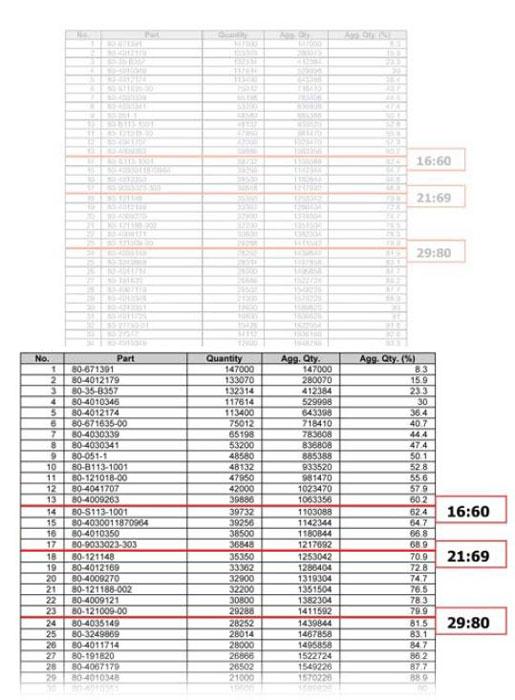
Figure 2
This shows input data for a shop’s 79 part numbers and their quantities, as well as the three ratio lines used in this PQ Analysis.
Figure 2 shows the parts sorted in order of decreasing quantity. Specifically, we need to determine what portion of the shop’s 79 part numbers make up 80, 70, and 60 percent of the operation’s aggregate quantity. Since part numbers cannot be divided in half, you will notice that some calculations result in the closest percentage possible to 60, 70, and 80.
So in this case, 13 part numbers (16 percent of the entire product mix of 79 part numbers) account for 60 percent of the total aggregate quantity; 17 part numbers (21 percent of 79) account for 69 percent of the total aggregate quantity; and 23 part numbers (29 percent of 79) account for 80 percent of the total aggregate quantity. This produces the following ratios: 16:60, 21:69, and 29:80, as shown in Figure 2.
So is this job shop a low-mix, high-volume operation, a high-mix, low-volume shop, or some combination of the two extremes? The numbers show the company actually is a combination of the two extremes. For the analysis, we use the 4:6, 3:7, and 2:8 ratios as guides. The 16:60 ratio is not close to that 4:6 ratio, but the 21:69 and 29:80 ratios are somewhat close to 3:7 and 2:8, respectively. Although this shop does have a significant percentage of part numbers tied to low volume, its medium- and high-volume parts represent the majority of what the shop actually produces. So in this case, we’ve chosen to divide the product mix into two segments, one comprised of the top 23 parts (corresponding to the 29:80 ratio line in Figure 2), and the other consisting of the remaining part numbers that are produced in significantly lower volumes.
Such an analysis can help focus data collection efforts. Job shops are complicated operations producing many products. This often makes continuous improvement efforts difficult, time-consuming, and costly, because collecting data for all products is so difficult.
Say that managers want to reduce material handling costs, standardize storage containers, and improve shop floor communications between machine operators and material handlers. This would require data collection to generate value stream maps, flow process charts, and material handling planning charts as part of a larger systematic handling analysis (SHA) initiative. Using the PQ Analysis, the improvement team could quickly select one (or more) products from the high-volume segment and leave the low-volume products for future investigation.
Working with only the high-volume segment, as identified in the PQ Analysis, the improvement team could produce a from-to chart to identify work centers that frequently process part numbers in the high-volume segment. Material handling cost boils down to the total time workers spend moving material between two locations. The time is a function of travel distance between the locations and the number of trips made between them (which is directly proportional to volume). In other words, the high-volume segment probably has the highest material handling costs.
Managers also can use the PQ Analysis to implement an inventory control policy that is suitable for each of the two (HMLV and LMHV) segments. Inventory control for the low-mix, high-volume runners could be done using supermarkets and kanban-based replenishment. In fact, if product families (based on common raw materials, sizes, or shapes) exist within that segment, then the improvement team could implement dedicated storage location, use of common containers and handling devices, and other inventory control measures. In contrast, inventory control for the high-mix, low-volume segment of parts would be done using a pure make-to-order strategy with zero on-hand inventory for these parts. In turn, this strategy would necessitate the use of finite capacity scheduling (FCS) based on due dates instead of the standard pull scheduling or MRP scheduling approaches.
While this approach may be a starting point, job shops shouldn’t stop here. Why? Because PQ Analysis does not consider the R (routings), $ (margin), and T (demand repeatability) of the product mix. As we have shown, the PQ Analysis method places importance on high-volume products. But for a job shop, a high-volume job may provide significant revenue and volume (Q), but at low margins ($).
In fact, it’s the R, $, and T information that really helps job shops hit the sweet spot in their business--that is, high profitability, which often means accepting complex, high-precision jobs with high-skilled-labor content that are produced in low volumes. Certain job shops tied to the defense and aerospace sectors, for instance, thrived during the worst of the recession because they managed to fulfill low-volume, high-margin orders for complex parts.
The next installment in this bimonthly series will add another layer to PQ Analysis: routings (R). PQR Analysis will show how to incorporate into the PQ Analysis the differences in a job shop’s part routings.
Future articles will focus on PQ$ Analysis, and PQ$T Analysis that, when combined with PQR Analysis, makes up our method, PQR$T Analysis, a method that has helped job shops achieve their lean goals, be flexible, and achieve high profitability.
This article is part of a series. For other articles in the series, click the following:
Analyzing products, demand, margins, and routings
Minding your P’s, Q’s, R’s--and revenue too
PQ$ Analysis: Why revenue matters in product mix segmentation


The Fabricator is North America's leading magazine for the metal forming and fabricating industry. The magazine delivers the news, technical articles, and case histories that enable fabricators to do their jobs more efficiently. The Fabricator has served the industry since 1970.
start your free subscription
Easily access valuable industry resources now with full access to the digital edition of The Fabricator.

Easily access valuable industry resources now with full access to the digital edition of The Welder.

Easily access valuable industry resources now with full access to the digital edition of The Tube and Pipe Journal.

Easily access valuable industry resources now with full access to the digital edition of The Fabricator en Español.
In this episode of The Fabricator Podcast, Caleb Chamberlain, co-founder and CEO of OSH Cut, discusses his company’s...