Minding your P’s, Q’s, R’s--and revenue too

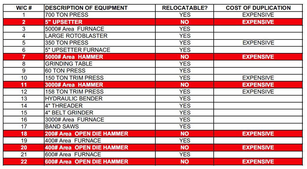
Figure 1
The company lists its work centers (W/Cs) and specifies whether the machine can be relocated and if the process would be expensive to duplicate. This is just a portion of the complete list of 57 work centers. The red signifies monuments, which aren’t practical to move. Highlighted green sections (not shown in this portion of the chart) signify outside processes.

This article is part of a series. For other articles in the series, click the following:

Analyzing products, demand, margins, and routings, Analyzing product mix and volumes: Useful but insufficient, PQ$ Analysis: Why revenue matters in product mix segmentation, Why a timeline analysis of order history matters

Most job shops, knowingly or unknowingly, operate multiple businesses under one roof. All these “businesses” use the same workforce, the same planning strategies, the same suppliers, the same facility layout, and the same equipment. In reality, job shop managers could split their product mix into two or more segments, and each segment ideally should be allocated a separate area and run using different management policies; support systems; workforce skills; and operational strategies, including scheduling, purchasing, inventory control, and facility layout. Why? It is because these segments share resources--including people and machines--and so inherently interfere and compete with each other.

As discussed in August, the PQ Analysis--relating product mix (P) to associated quantities (Q)--is a useful but incomplete method for segmenting the product mix of a job shop. Yes, it is simple to implement on a spreadsheet, and it complements value stream mapping (VSM). Although VSM and the PQ Analysis complement each other, both are really effective only in low-mix, high-volume situations. This method incorrectly focuses attention on a small percentage of a job shop’s product mix. Worse, it fails to consider the routing, revenue, stability, and repeatability of demand for a job shop’s different products. VSM works best in low-mix, high-volume assembly facilities. In fact, the fundamental concept of VSM is based on the theory of assembly line balancing--and an assembly line simply is not a job shop, and never will be. VSM can map a single or, at best, two or three routings, which is obviously not enough for a job shop. Nor have I seen VSM able to depict an entire family of products with different setups and cycle times for various operations in their routings.

Essentially, VSM is a method that misleads job shops into believing that, just because they have a few high-volume products, their entire business can run to the assembly line-like “beat” of repetitious production. This is why the PQR$T Analysis can play a valuable role--it reflects the realities job shop managers face. They have a diverse product mix (P) with different routings (R) produced in various quantities (Q) with varying revenue and profits ($) and demand stability and order repeatability (T). Analyzing all these factors helps shop managers see the whole picture.Analyzing Products and Routings

In this column I describe an approach that incorporates a PR Analysis (one relating product mix and routing similarities) into a PQ Analysis, creating the PQR Analysis. I also show the benefits of a PQ$ Analysis, which brings revenue into the decision-making. Although not as comprehensive as the complete method of PQR$T Analysis, the product-quantity-routing-revenue (PQR$) analysis, will surely not mislead job shop owners about their product mix, as does the PQ Analysis.

The PQR Analysis segments a product mix into at least two, three, or more segments. Thereafter, product families in each segment can be produced using a suitable manufacturing system, be it a high-volume cell devoted to a single product; a flexible line devoted to a product family; or a flexible cell that, say, can run unattended overnight to produce a large family of parts, but during the day produce the remaining low-volume products in the product mix.

Much of the methodology behind PQR Analysis comes from the Production Flow Analysis (PFA) work of Prof. John Burbidge of Britain, as well as the Group Technology strategies that helped transform numerous job shops in the U.K. into cell-based facilities during the 1970s. These proven approaches for high-mix, low-volume manufacturing were pioneered by the British, Germans, and Russians--and not Toyota. The Toyota Production System provides significant value for high-volume, low-mix production. But a job shop, of course, is not Toyota.

The Analysis

Consider one job shop that has 530 products with routings using 57 pieces of equipment (work centers), including equipment available at the shop’s suppliers. Like any contract manufacturer, it’s a complex, highly variable operation.

The shop uses analytical software to compute the current state of affairs. In this example, the company uses the Production Flow Analysis and Simplification Toolkit (PFAST) from The Ohio State University, but it may well be possible to implement these same analytics using Microsoft Excel® or Access®, or even Six Sigma statistical analysis software such as Minitab®.

To start, the improvement team assigns each work center (W/C) a number and determines whether the machine is a monument or if it can be relocated (see Figure 1). They determine if the process would be expensive to duplicate if the shop wanted to purchase new machines to minimize shared resources among product-mix segments.

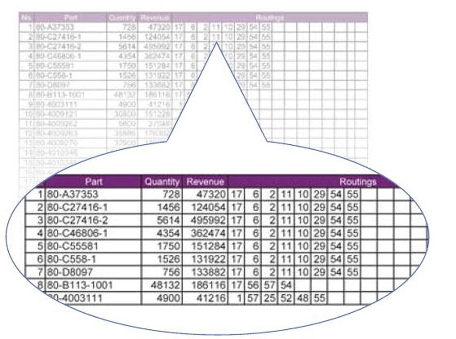
Figure 2
This spreadsheet shows the input data used for PQR$ Analysis; that is, quantity (Q), revenue ($), and the routing (R) for each product/part (P). Note, this is just a sample of parts that was extracted from the product mix of 530 part numbers, as described later. A complete PQR Analysis would include all 530 part numbers--and analyzing all product routings does have value, as revealed in the “Narrowing the Analysis” section.

The team also produces the information in Figure 2, which shows the quantity, routing (with corresponding W/C numbers), and revenue for each product number over a specified period. Figure 3 shows the current facility layout with all the W/C locations, including unmovable monuments.

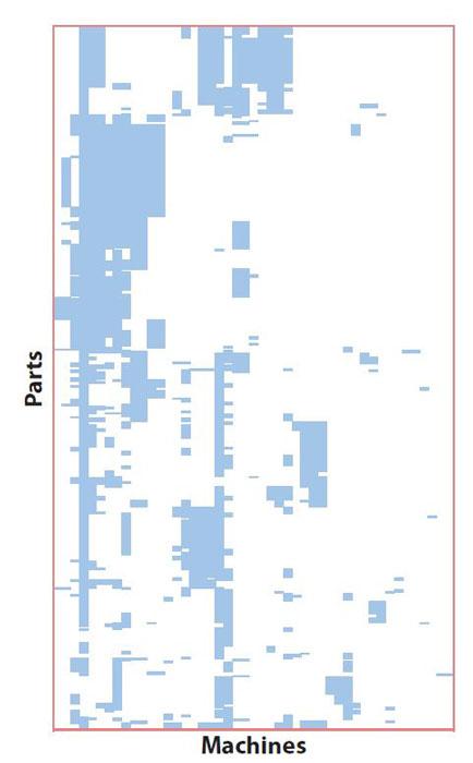
Next the shop analyzes all 530 products and their individual routings to assess if there are families of parts using groups of machines that could be moved into manufacturing cells. From here they develop a full-scale PR Analysis (see Figure 4), also called a machine-part matrix clustering or product-process matrix clustering. Think of this analysis as a visualization of all 530 value streams without using VSM at all.

At every point a part number along the Y axis (a row in the spreadsheet) is matched with a work center along the X axis (a column in the spreadsheet), a “1” is placed. Compact blocks of 1s suggest part families are present. Note that Figure 4 is a 530-line chart miniaturized, so clusters of 1s appear as solid blue blocks.

Narrowing the Analysis

Working with all 530 part numbers at once isn’t practical for any improvement effort. So from here the team extracts a smaller sample of part numbers that have significant volume, significant revenue, or share common routings. Here is where analyzing the product mix (P), quantities (Q), routings (R), and revenue ($) comes into play. This is where the team also uses the PFAST software to replace the traditional PQ Analysis of the entire product mix with a PQ$ Analysis.

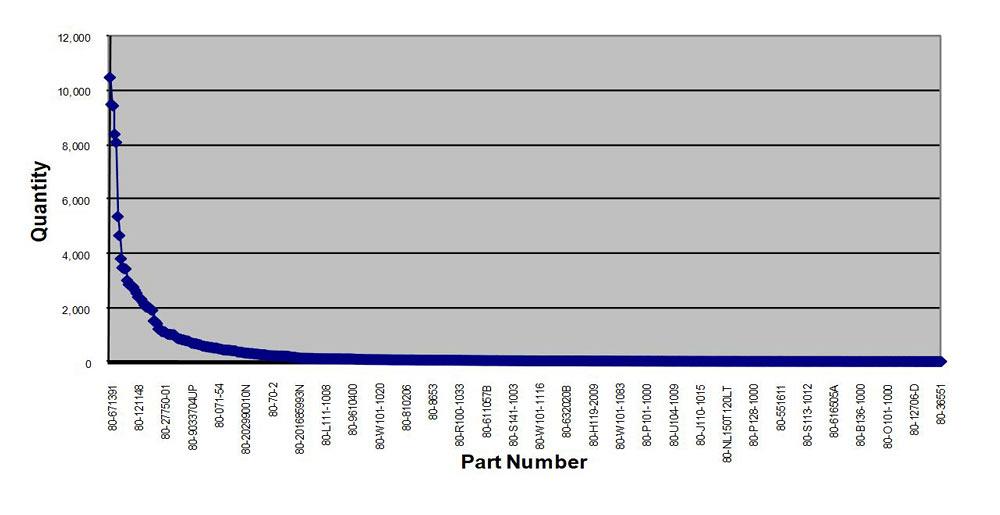
Figure 5 shows a typical PQ Analysis distribution of production volumes for a job shop. The head on the left side of the graph shows the few product numbers with high volumes, while the long tail to the right shows numerous jobs with low volumes.

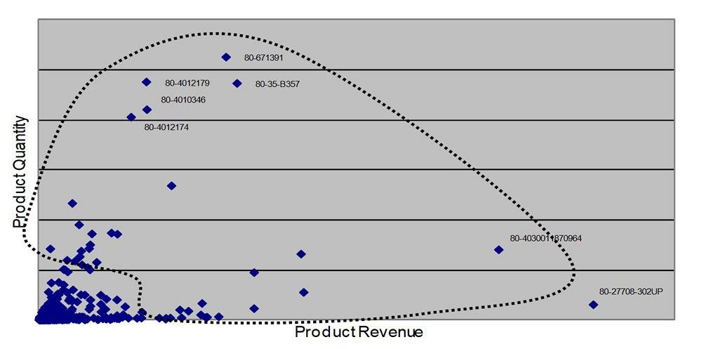
Figure 6 brings revenue into the mix. As shown, most jobs have low quantities and low revenue--no surprises there. But note the remaining jobs. A few high-quantity jobs produce only moderate levels of revenue, while a significant number of low-quantity jobs produce moderate and even high revenue.

Considering both part quantity and revenue, the team focuses on products produced in quantities greater than 1,800 and earning revenue of more than $30,000, as shown by the dotted line in Figure 6. Initially only 44 product numbers were included in the sample, which accounts for only about 8 percent of the total product mix, 68 percent of the total volume, and 46 percent of the total revenue. In other words, almost half of the company’s earnings come from those 44 products.

Here is where that original, complete PQR Analysis in Figure 4 steps back into the picture. Of the hundreds of remaining products not included in the sample, 35 have routings similar or identical to a significant number of routings for the 44 products initially selected in the sample. Seeing this, the team decides to include them in the sample selected for improvement, bringing the total number of products to 79--or 15 percent of the total number of active products, about 74 percent of the total volume, and about 54 percent of the total revenue.

Analyzing the Sample

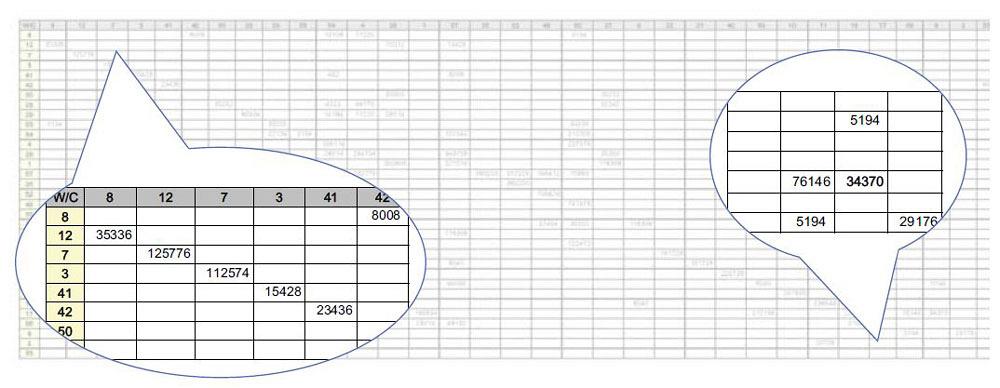
These steps narrow the analysis and determine which products use similar machines, but they do not truly reveal the complex material flow that plagues the job shop. So from here the team uses the product mix, quantity, and routing information for the 79 products in the sample to develop a “from-to” chart (see Figure 7).

The chart lists the same set of work centers in the same sequence on both the X and Y axes. Software breaks up each routing into several from-to segments--that is, the quantity of products that move from one specific W/C to another. If a part goes from W/C 17 to 6, 2, 11 and so on, the software will split this into “from-to” segments: 17 to 6, 6 to 2, 2 to 11, and so forth. Note that this analysis then has to be repeated for each of the 79 routings in the sample. (Not surprisingly, job shops shy away from doing such crucial analysis because of the tedium and inherent error of data mining by hand.)

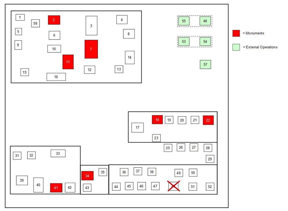
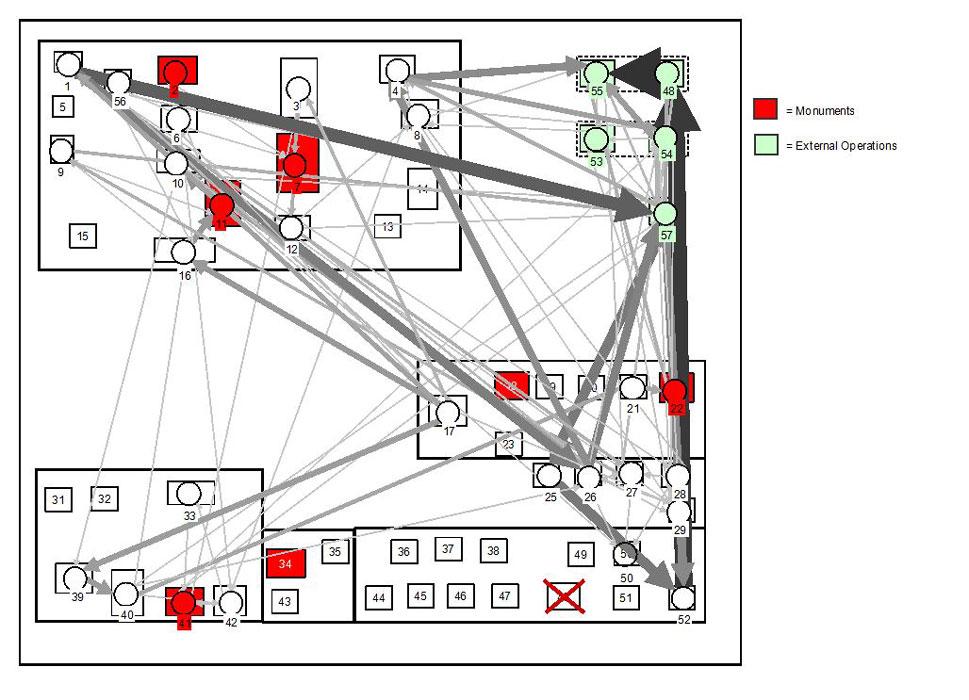
Figure 3
The current shop layout shows monuments in red, external operations in green.

For instance, Part No. 80-A37353 has a quantity of 728. The routing starts at W/C 17 and moves to W/C 6--that is, from the band saw to the furnace--before moving to other operations downstream. In this case, the quantity of 728 is inserted where W/C 17 (on the Y axis) and 6 (on the X axis) intersect, as shown in Figure 7. When this 728 is added to the quantities from all part numbers flowing between those machines, the chart reveals that, during a predetermined time period, 34,370 workpieces travel from the band saw (W/C 17) to the furnace (W/C 6).

When the flow volumes and directions between all pairs of work centers are superimposed on the facility layout, with arrow thicknesses proportional to traffic volumes, the result is the flow diagram in Figure 8. The chaos in this diagram is common for job shops.

Identifying Product Families

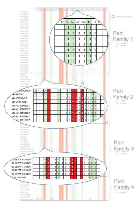
After analyzing the part routings using one of the four PR Analysis algorithms available in PFAST software, the team organizes the 79 part numbers into four product families, as shown in Figure 9. The clusters of 1s indicate products with similar routings using the same W/Cs.

In Figure 3 the blocks colored red correspond to the W/Cs that are monuments, and the blocks colored green correspond to outside operations (vendors and the company’s own machine shop located several miles away). Figure 9 uses the same color scheme--red for monuments and green for outside processes.

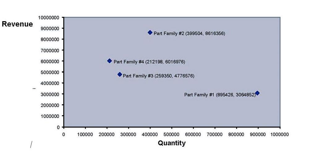
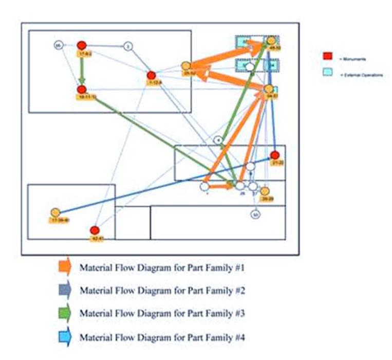
Using the results of Figure 9, the company develops a scatter plot depicted in Figure 10 to compare the four part families with each other, based on the total quantity (Y axis) and the total revenue (X axis). Then they develop another material flow diagram, as shown in Figure 11, that superimposes the material flow diagrams for each of the four part families on each other.

The Payoff

Seeing all this, could this shop be organized into four product family cells? Probably not, especially considering the number of monuments in part families 2 and 3 (again, those columns marked in red), although at least the first part family could be produced in a dedicated cell. Regardless, the analysis gives a clear picture of the current, albeit complex, state of affairs on the shop floor.

At first glance, all this may seem like a lot of effort for not much reward. But this analysis is just a starting point. It gives the improvement teams a guide, showing what to tackle first and which strategies would pay off, as well as which ideas to avoid.

The actual job shop in this example moved certain machines to reduce job travel time and purchased other equipment to make material flow more efficiently. Ultimately, the resulting throughput increase saved $137,000 a year. That’s not a bad return on investment.

Slide Show | 11 Images