PQ$ Analysis: Why revenue matters in product mix segmentation

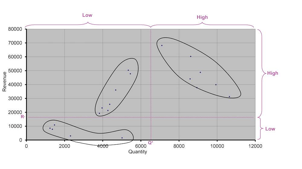
Figure 1
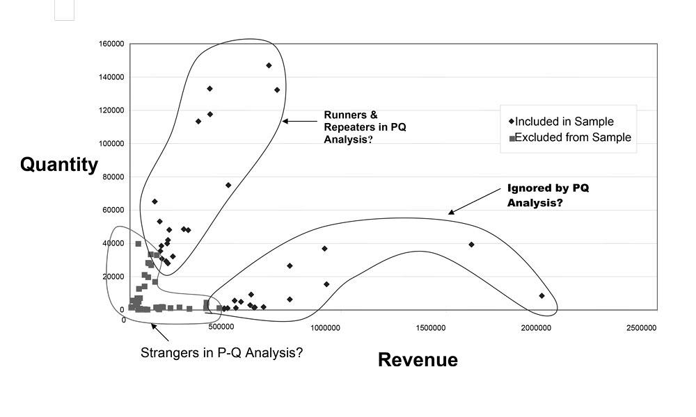
This PQ$ Analysis scatter plot shows the product mix of a hypothetical job shop.

Job shops serve various business sectors that demand different parts or products in specific quantities or production volumes. Developing an improvement road map requires managers to analyze this product mix using a multicriterion approach like the PQR$T Analysis. Each criterion used to develop the analysis is critical. Considering only product quantities, as in a traditional PQ Analysis, would produce vastly different results--and may point job shops in the wrong direction when it comes to continuous improvement.

That is because a traditional PQ Analysis considers the mix of parts (P) and their quantities (Q). Unfortunately, such an analysis identifies--at most--only three product segments: high, medium, and low volumes. The PQ Analysis runs into problems when applied to high-mix, low-volume manufacturing, especially job shops that produce small batches of high-priced products. The PQ Analysis ignores these low-volume products, even though they may bring in significant revenue. At the same time, it may emphasize certain high-volume jobs that are not big money-makers.

Any business can improve cash flow by completing high-value orders in the shortest period of time, and by minimizing lean manufacturing’s seven types of waste that decrease profitability of low-volume products that have, or could have, very healthy margins. From the perspective of part flow, three types of operational costs--transportation, work-in-process, and queuing--increase manufacturing costs. Two of those costs--transportation and queuing--depend heavily on production volumes and container sizes, but WIP costs depend heavily on product value, which is usually reflected in the sales earned from each product.

This is where PQ$ (Product-Quantity-Revenue) Analysis can help. Instead of focusing on a sample of products selected using a single criterion--quantity--this analysis brings revenue into the equation. Most important, it does not just separate the product mix based on volume (low, medium, or high), but into at least four segments. For instance, if a shop decides to separate products into high and low categories on both criteria (volume and revenue), then every product would fall into one of the following four segments: high-volume, high-revenue; low-volume, high-revenue; high-volume, low-revenue; and high-volume, high-revenue. If a shop were to categorize each criterion into low, medium, and high categories, the number of segments would, of course, grow to nine, and so on.

The bottom line: PQ$ Analysis incorporates how much money parts actually make. And when it comes to running a business, two things matter: The total amount of money made, and the speed with which those orders that make the most money are completed and shipped.

The PQ$ Analysis produces a scatter plot, as shown in Figure 1. The horizontal axis (X) represents quantity or volume, while the vertical axis (Y) represents revenue, or profit margin. Every point in the scatter plot represents a particular product. As Figure 1 shows, this shop’s product mix appears to have only three segments: low-quantity, low-revenue; low-quantity, high-revenue; and high-quantity, high-revenue.

The dotted lines on the two axes are threshold values, separating low revenue from high revenue (R*) as well as low from high quantities (Q*). Each quadrant defines a product mix segment that ideally should be managed as a separate business and be produced in a separate area of the facility with a suitable layout, as well as distinct manufacturing technology and workforce skills.

Whole Greater Than the Parts

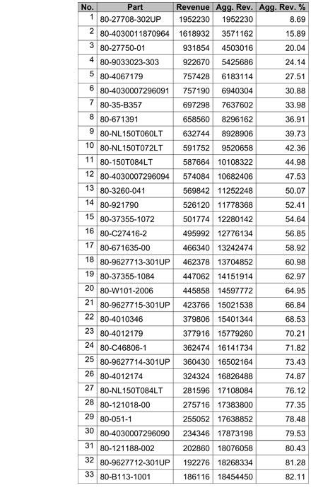
Figure 2 shows how a typical job shop would prioritize products based only on quantity. Part numbers that run in the highest volumes are placed on top, followed by part numbers with decreasing quantities.

The PQ Analysis curve in Figure 3 shows that the shop runs few part numbers in high quantities. In fact, most parts run in low quantities, as shown by the long tail--typical for a job shop. The line’s sharp curve indicates a potential cutoff point between different product mix segments--that is, between low-volume “strangers,” medium-volume “repeaters,” and high-volume “runners.” The shop uses the Pareto principle, or 80-20 rule, to separate products into two segments: the top 23 part numbers represent the high-volume segment (representing 80 percent of aggregate volume), and the remaining 56 part numbers represent the low-volume segment.

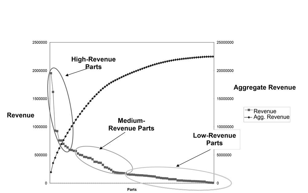
But what about revenue? To include that variable, a P$ Analysis replaces quantity with revenue to produce the chart in Figure 4, which ranks part numbers from highest to lowest sales dollars. Next, a threshold line is inserted between the “high-revenue” and “low-revenue” segments by using the 80-20 rule as a guide, grouping the top-sales-dollar parts that produce 80 percent of total shop revenue. This produces the scatter plot in Figure 5.

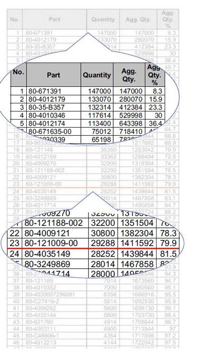
Figure 2
In a PQ Analysis, products are ranked by quantity, with the highest-volume products on top. The red line indicates the threshold between the high-volume and low-volume segments of the product mix.

Are the two parts samples--the high-quantity parts from the PQ Analysis and the high-revenue parts from the P$ Analysis --the same? No! By using PQ$ Analysis, the shop is able to incorporate both quantity and revenue in the analysis, producing the scatter plot in Figure 6, which suggests that the product mix could be broken into three segments: high-volume, low-revenue; low-volume, high-revenue; and low-volume, low-revenue.

The part groupings are distinct enough that we could actually just eyeball them to get a general idea of which products should be part of which segment. But to be more precise, we simply locate the point on the scatter plot that represents the product number corresponding to the revenue threshold, R*, where aggregate revenue reaches 80 percent, and draw a vertical line. We would do the same with quantity, Q*, to draw a horizontal line, as was shown earlier in Figure 1.

Note that if the shop had relied solely on the PQ Analysis, it would have ignored products in the high-revenue, low-volume segment. And if managers relied only on the P$ Analysis, they would have ignored the low-revenue, high-volume segment. It is important that job shops remember that lean for them is about doing whatever will make them flexible, agile, and reconfigurable and reduce costs through waste elimination.

Using the Analysis

So how can this information guide improvement projects such as kaizen events, management policies, and strategic planning? Some examples follow.

Market Diversification. Figure 6 shows that this hypothetical job shop does not have a single part in the high-revenue, high-quantity quadrant. That’s typical, because job shops do not specialize in high-volume, low-mix manufacturing. However, managers probably wouldn’t want to pass up a long-term contract from a defense prime contractor or OEM to supply a single part or well-defined part family, ordered on a consistent basis throughout the year--perhaps even for a few years. In this case, the shop could apply many lean elements to these types of jobs, including determining a takt time to sync production with that rarity in the job shop world: consistent customer demand.

Facility Layout and Workforce Training to Operate Virtual Cells. A manufacturer of hydraulic pipes and couplings produces 2,000 SKUs, all requiring a 48-hour lead-time. The company, however, was finding it increasingly difficult and costly to achieve this lead-time. An analysis showed that more than half of sales came from only 92 products--or less than 5 percent of the entire product mix. Customers ordered other products infrequently in small quantities, even as single items.

Armed with this information, managers decided the company needed two types of factories: a high-volume, repetitive manufacturing facility and a flexible job shop. However, it was not cost-effective to build two factories or even to physically separate the equipment. Instead, managers determined what equipment would be needed for high-volume products in a fixed sequence and painted those machines green. To determine who would run these machines, managers selected employees based on their work routine preference and gave them green overalls. They painted the remaining equipment beige and selected employees who preferred to tackle difficult and complex operations, including frequent setups--and, yes, gave them beige overalls.

Although the equipment and staff intermingled on the floor, each business operated totally differently. The green factory had fixed hours of work, just-in-time deliveries, and improvement activities focused on achieving faster cycle times and increased productivity. The beige factory had work hours that varied according to the level of demand each week. Materials were purchased only when required. Improvement activities focused on flexibility and responsiveness. This company succeeded in creating and operating two businesses under the same roof, even if each business had different policies, procedures, and performance metrics.*

Vendor Selection and Purchasing Management. High-volume products, which allow production batch sizes to match a make-to-stock inventory policy, influence how far the suppliers are from the company location. Low-volume operations work well with nearby suppliers, so they can deliver partial truckloads quickly; while high-volume, consistently demanded products allow for more distant suppliers to make periodic, full-truckload deliveries, because such deliveries (like production) are relatively consistent and predictable. No manufacturer wants a long and dispersed supplier network.

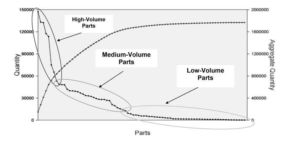
Figure 3
The PQ Analysis shows that the shop runs a few high-volume parts, and has a “long tail” of various low-volume parts. This is typical for job shops.

In contrast, high-revenue, low-volume products, many of which comprise less common materials, may require a different purchasing and inventory strategy. For instance, a product containing titanium--which is not easily available if shipped from, say, China--merits a close watch on available inventory, supplier lead-times, and market prices. Bulk purchases that earn quantity discounts would be the right thing to do, even though traditional lean thinking considers this as “inventory waste.”

Inventory Control and Scheduling. Specific inventory control systems can be used for products in different segments. Consider products in the high-volume, low-revenue segment. These orders could help develop customer relationships. In fact, the same customers may also provide valuable high-revenue orders. Still, why should a job shop focus improvement efforts on large orders that don’t make much money? In this case, a shop could outsource low-revenue, high-volume jobs to another company. The job shop would simply receive the parts from the subcontractor, label them, and ship them to the end customer. True, because the job shop outsources these orders, margins may suffer--but these orders already have low margins to begin with. Removing this work from the shop floor would focus the time and money invested in continuous improvement on other parts in the product mix, which would lead to a healthier balance sheet.

For shop floor scheduling, the color of the paperwork and containers associated with a high-revenue order could be different from the paperwork for the other orders. This way, everybody gives a higher priority to minimizing WIP contributed by those high-revenue items that have to wait in queues at different work centers across the facility.

Equipment Purchases. The value and volume of production of different products influence the flexibility and sophistication of manufacturing equipment. High-volume assembly facilities are increasingly embracing “right-sized” automation--that is, equipment designed for producing well-defined products in a well-defined range of volumes. On the other hand, many job shops that struggle to hire and retain skilled equipment operators are the first to purchase flexible, multifunction, single-setup machines, some capable of lights-out operation.

Demand Repeatability and Stability

A complete product mix segmentation analysis involves one final element: demand over time, the “T” in PQR$T Analysis. The PQ Analysis, based on the 80-20 rule, fails to consider how many times a product is ordered, the size and variability of those orders, and the time interval between consecutive orders. This is why the PQT Analysis is preferred for identifying the runners (high volume, frequently ordered), repeaters (medium volume), and strangers (low volume, rarely ordered) in a job shop’s product mix.

For other articles in this series, see the following:

Analyzing products, demand, margins, and routings

Analyzing product mix and volumes: Useful but insufficient

Minding your P’s, Q’s, R’s--and revenue too

Why a timeline analysis of order history matters

Slide Show | 6 Images